
References
Home
Toolbar
Expressions
Time Format
Preferences
Import
Perl Import Filter
Perl Data Filter
Command Line
Inspectors
Attribute Inspector
Data Buffer
Data
MySQL
Curve Fit
Macro
Macro
Miscellaneous
Search
Curve Fit Inspector
This function allows you to fit data with some predefined functions or free defined functions. Fits are possible with up to 24 functions each with up to 5 free parameters.
To start a fit two things are necessary. 1. the function(s) you will fit and 2. the start parameters for the function(s). Fitting will only work if the function you provide will match the data of your buffer otherwise the fit will not succeed and you will see an error message. Fitting work better the closer the start parameters match the data.
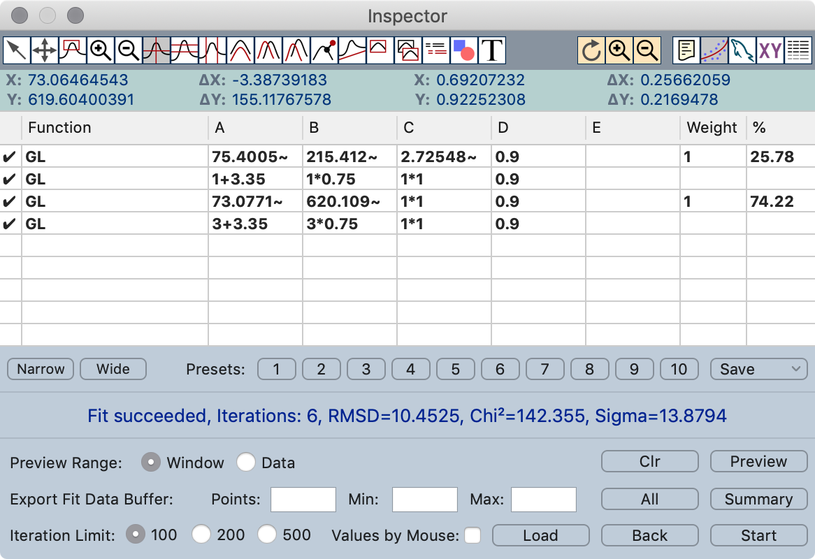
The Curve Fit Inspector consists of a few controls and a table for the function and fit parameter definition.
Function Table
Active functions are displayed with a check mark in the first column. Double clicking the first column changes the state.
Function: In this column you have to define the function you want to fit (see below).
A, B, C, D, E: This are the free parameters for the fit function.
Weight: The weight of a function for the integration routine (only used by the special functions).
%: The result of the integration will be displayed in this column (only calculated for the special functions).
Controls
Narrow/Wide: Change fit table layout to narrow/wide columns.
Presets 1-10: Load a stored curve fit preset.
Save: Save the current cure fit parameter as one of the 10 possible presets.
Preview: Displays all the fit functions and the summary curve in the current document.
Clr: Clear the fit preview.
Preview Range: Define if the preview should cover the range of your data or the window range. This apply also to export if no export range is defined.
Export Fit Data Buffer: Allows to export fit results as new buffers to the document.
Iteration Limit: Defines a cycle limit after which it is possible to stop the fit.
Values by Mouse: If this button is checked the values from the mouse mode Measure will be sent to the currently selected line in the parameter table (A = X position and B = Y position). After this the next line in the parameter table will selected automatically. This makes it easy to predefine a bunch of peaks.
Load: Loads fit data from another document.
Back: Every time you start a fit the state will be saved in a history buffer. With this button you can go back trough the fit steps.
Start: Starts the fit for the current working buffer.
Fit result
The text field in the middle of the inspector shows the status and the result of the fit. The first line displays the fit state and the second the fit result:
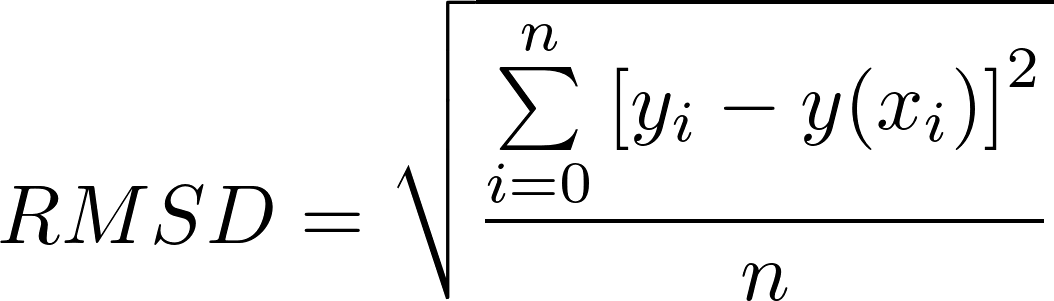
RMSD: Root mean square deviation of the last cycle:
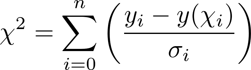
Chi²:
Function definition
In the Function column you can enter normal mathematical expression as functions for fit (there are some special functions, see below).
Available variables:
| x | x value |
| A | A parameter |
| B | B parameter |
| C | C parameter |
| D | D parameter |
| E | E parameter |
Example: (x+A)^2+B
For the 5 fit parameter (A,B,C,D,E) the following syntax is possible:
| <value> | a fixed value |
| <value>~ | a value which should be fitted |
| <value>~<dvalue> | a value which should be fitted in the range from <value> - <dvalue> to <value> + <dvalue> |
| <row>[+,-,*,/]<rel> | sets value in relation to an entry of same column in a previous row |
Examples: 284 1234~ 10.7~0.2 1-2.3 5*0.12
Special Functions
The fit function supports some special functions. These functions are easy to use and a little bit faster than free defined functions. The special functions can not be used together with other expressions in one row.
GL (Gauss-Lorentz mix curve)
B = height (I0)
C = width ( α, FWHM)
D = Gauss-Lorentz ratio ( M ,1.0=pure Gauss, 0.0 = pure Lorentz)
E = unused
DS (Doniach-Sunjic curve)
B = height (l0)
C = width ( γ, Lorentzian FWHM)
D = Anderson's exponent ( α, -0.5 ... 0.5)
E = unused
ET (Gauss-Lorentz mix curve with exponential Tail)
B = height (I0)
C = width ( γ, Lorentzian FWHM)
D = Gauss-Lorentz ratio ( M ,1.0=pure Gauss, 0.0 = pure Lorentz)
E = tail exponent factor ( α, -infinity - +infinity)
GL* (Gauss convoluted Lorentz curve)
B = height
C = width (FWHM)
D = Gauss-Lorentz ratio (must be set to 0.0)
E = Gauss FWHM (0 - +infinity)
DS* (Gauss convoluted Doniach-Sunjic curve)
B = height
C = width (Lorentzian FWHM)
D = Anderson's exponent (-0.5 ... 0.5)
E = Gauss FWHM (0 - +infinity)